개요 및 전체 데이터 모델 설명
application_train(test) 주요 속성 분류
- 대출 금액
- 고객 신상
- 고객자산
- 고객 소득
- 고객 거주지
- 고객 행동 : 인지심리학적인
Label Encoding vs. onehot Encoding
lightGBM에서는 피처들이 너무 많기 때문에, 성능을 크게 향상시켜주는것 같진 않음
LightGBM,XGBoost는 널값을 자동으로 처리해
💡
없는 피처들을 만드는게 중요.(고객 행동 같은, 데이터 수집 요청, 프로모션 같은 것들을 직접 얻어야함)
1. 라이브러리와 APP 데이터 세트 로딩
Copy
import numpy as np
import pandas as pd
import gc
import time
import matplotlib.pyplot as plt
import seaborn as sns
#import warning
%matplotlib inline

#warning.ignorewarning(...)

pd.set_option('display.max_rows', 100)
pd.set_option('display.max_columns', 200)- target값 분포 및 amt_imcome_total값 histogram
Copy
app_train['AMT_CREDIT'].hist()
#plt.hist(app_train['AMT_INCOME_TOTAL'])
- AMT_INCOME_TOTAL이 1000000이하인 값에 대한 분포도
Copy
# boolean indexing 으로 filtering 적용
app_train[app_train['AMT_INCOME_TOTAL'] < 1000000]['AMT_INCOME_TOTAL'].hist()
Copy
# distplot으로 histogram 표현
sns.distplot(app_train[app_train['AMT_CREDIT'] < 1000000]['AMT_CREDIT'])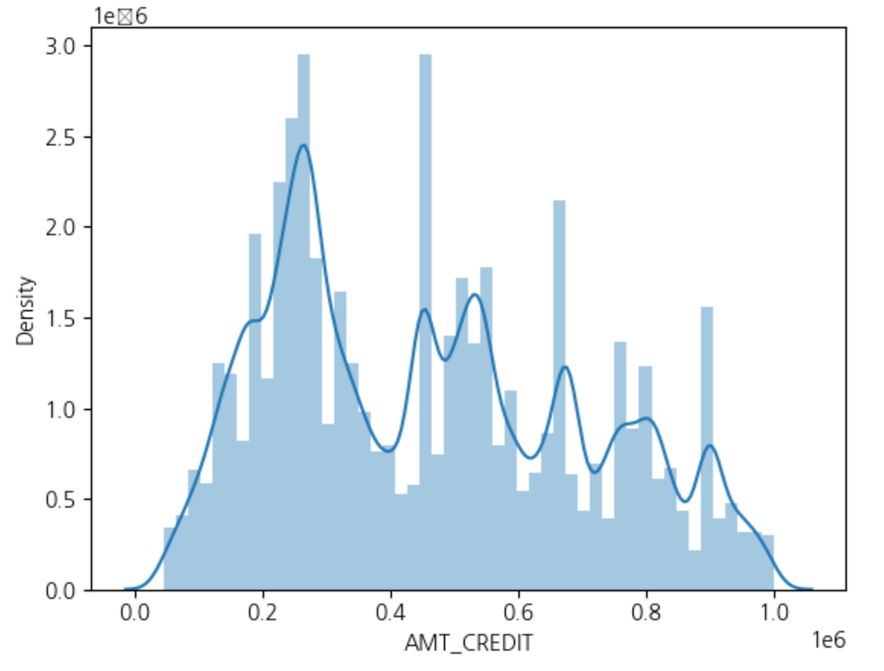
- target값에 따른 amt_income_total값 분포도 비교
Copy
# TARGET값에 따른 Filtering 조건 각각 설정.
cond1 = (app_train['TARGET'] == 1)
cond0 = (app_train['TARGET'] == 0)
# AMT_INCOME_TOTAL은 매우 큰 값이 있으므로 이는 제외.
cond_amt = (app_train['AMT_INCOME_TOTAL'] < 500000)
# distplot으로 TARGET=1이면 빨간색으로, 0이면 푸른색으로 Histogram 표현
sns.distplot(app_train[cond0 & cond_amt]['AMT_INCOME_TOTAL'], label='0', color='blue')
sns.distplot(app_train[cond1 & cond_amt]['AMT_INCOME_TOTAL'], label='1', color='red')
- Violinplot을 이용하면 category별로 연속형 값의 분포도를 알수 있따.
Copy
# violinplot을 이용하면 Category 값별로 연속형 값의 분포도를 알수 있음. x는 category컬럼, y는 연속형 컬럼
sns.violinplot(x='TARGET', y='AMT_INCOME_TOTAL', data=app_train[cond_amt])ㄴ
- app_trian과 app_test를 합쳐서 한번에 데이터 preprocessing 수행.
Copy
# pandas의 concat()을 이용하여 app_train과 app_test를 결합
apps = pd.concat([app_train, app_test])
apps.shape- Object feature들을 Label Encoding
- Null값 일괄 변환
Copy
apps.isnull().sum().head(100)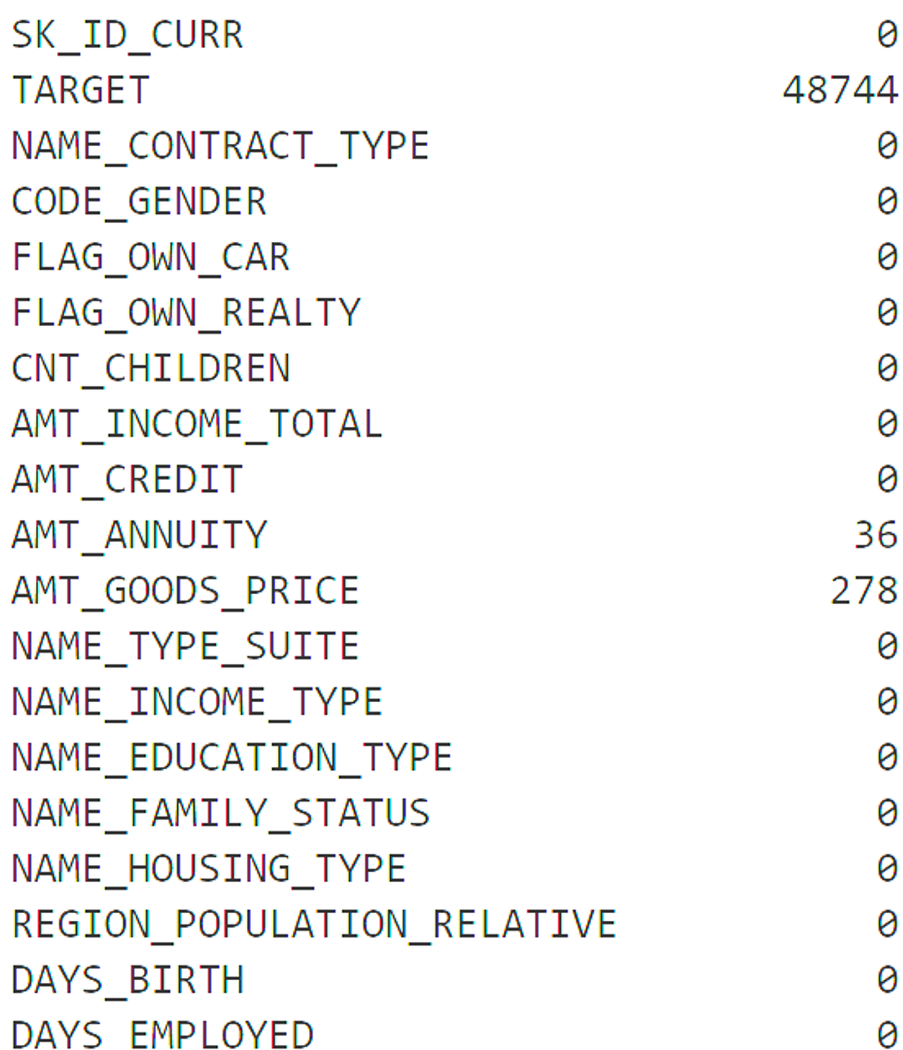
- 학습 데이터를 검증 데이터로 분리하고 LGBM Classifier로 학습 수행
Copy
ftr_app = app_train.drop(['SK_ID_CURR', 'TARGET'], axis=1)
target_app = app_train['TARGET']
Copy
from sklearn.model_selection import train_test_split

train_x, valid_x, train_y, valid_y = train_test_split(ftr_app, target_app, test_size=0.3, random_state=2020)
train_x.shape, valid_x.shape
Copy
from lightgbm import LGBMClassifier

clf = LGBMClassifier(
        n_jobs=-1,
        n_estimators=1000,
        learning_rate=0.02,
        num_leaves=32,
        subsample=0.8,
        max_depth=12,
        silent=-1,
        verbose=-1
        )

clf.fit(train_x, train_y, eval_set=[(train_x, train_y), (valid_x, valid_y)],
eval_metric= 'auc', verbose= 100, early_stopping_rounds= 50)- Feature importance 시각화
Copy
from lightgbm import plot_importance

plot_importance(clf, figsize=(16, 32))
- 학습된 Classifier를 이용, 테스트 데이터를 예측
Copy
#학습된 classifier의 predict_proba()를 이용하여 binary classification에서 1이될 확률만 추출
preds = clf.predict_proba(app_test.drop(['SK_ID_CURR'], axis=1))[:, 1 ]
'Python' 카테고리의 다른 글
| 파이썬 기초 - 01_과목평균 (0) | 2024.08.17 |
|---|---|
| Pytorch 튜토리얼 - 텐서연산 및 신경망 구성 (1) | 2024.08.16 |
| 분류(Classification) - 3 베이지안 최적화와 고객만족예측 실습 (2) | 2024.07.23 |
| 분류(Classification) - 2 (2) | 2024.07.20 |
| 분류(Classification) - 1 (0) | 2024.07.17 |